What is Deep Learning?
Deep learning is a subset of machine learning that includes training artificial neural networks with multiple layers to learn and make predictions or decisions based on input data. In deep learning, the neural network is designed to recognize patterns in large datasets by using algorithms to identify relationships between different variables. The term “deep” generally refers to the number of layers in the neural network, which can range from ten to even thousands. These neurons help process the input data and make the output.
Why Deep Learning Now?
The term learning speaks for itself. Learning involves training. To train a model, we need data. In this day and age, data is available everywhere on the internet. Quality data is easier to get now than ever before. This training is not easy either. Many mathematical computations are done every second during the traning phase. To compute this, we need a significant amount of computation power. The rise of powerful GPU and CPU has made it easier. Some GPUs are designed specifically for training models. Software is not far behind in this regard. Programming languages like Python and libraries like PyTorch, TensorFlow, etc. have made it 100 times easier to make a model.
Perceptron
A deep learning model is made with thousands, if not millions, of neurons. A single neuron is called perceptron.

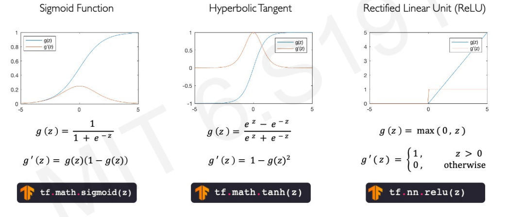
A perceptron takes an input mutiplied with weight then we add it. That addition is added with a bias which is a scaler weight. Then it is passed through a non linear activation function. But why non linear activation function? It is because real world data are mostly non linear. And to calculate non linearity we need a non linear function. Bias here helps to shift the non linear activation function. There are many non linear activation function. One of the popular one is sigmoid function. It takes any any number as input in real number line and gives output 0 to 1 likely a threshold function. Some more popular non linear activation functions are Hyperbolic Tangent and Rectified Linear Unit.
Loss function
In deep learning, the goal is to use a neural network to approximate a function that maps input data to output values. This approximation is learned by minimizing a loss function using a technique called backpropagation. the loss function is first computed for a given input to the network and then the gradient of the loss function with respect to each parameter in the network is calculated using the chain rule of calculus.
The gradients are then propagated back through the layers of the network, starting from the output layer and moving backwards towards the input layer. At each layer, the gradients are used to update the parameters of the layer using an optimization algorithm such as stochastic gradient descent.
By iteratively updating the parameters of the network using backpropagation, we can minimize the loss function and train the network to make accurate predictions on new data. In machine learning, the loss function is a measure of how well a model’s predictions match the ground truth (actual) values. The goal during training is to minimize this loss function, which results in the model making more accurate predictions.
One commonly used loss function for classification problems is softmax cross-entropy. This loss function is typically used when the output of the model is a probability distribution over multiple classes.
The softmax function takes a vector of arbitrary real-valued scores and squashes it into a vector of probabilities that add up to 1. The softmax function is defined as:
$$ \text{softmax}(z_i) = \frac{\exp(z_i)}{\sum_j \exp(z_j)} $$
where $z$ is a vector of real-valued scores, and $i$ and $j$ are indices that iterate over the elements of the vector.
The cross-entropy loss function measures the difference between the predicted probability distribution and the true probability distribution. It is given by:
$$ \mathcal{L} = -\sum_{i=1}^{n} y_{i} \log(\hat{y}_{i}) $$
where $n$ is the number of classes, $y$ is a one-hot encoded vector representing the true class label, and $\hat{y}$ is the predicted probability distribution over the classes.
To understand this equation, let’s consider an example. Suppose we have a classification problem with three classes, labeled A, B, and C. We want to predict the probability of each class given some input data. Let’s say our model predicts the following probabilities:
$$ \hat{y} = [0.3, 0.4, 0.3] $$
and the true label is B. We can represent the true label as a one-hot encoded vector:
$$ y = [0, 1, 0] $$
Using the softmax cross-entropy loss function, we can compute the loss as follows:
$$ \begin{align} \mathcal{L} &= -\sum_{i=1}^{3} y_i \log(\hat{y}_i) \ &= -[0 \cdot \log(0.3) + 1 \cdot \log(0.4) + 0 \cdot \log(0.3)] \ &= -\log(0.4) \ &= 0.916 \end{align} $$
The goal of training is to minimize this loss function by adjusting the parameters of the model. By computing the gradients of the loss function with respect to the model parameters using backpropagation, we can update the parameters and improve the model’s accuracy.